Discovering PixelMath
This tutorial is aimed at introducing the latest tool to handle images, developed in Siril 1.0.0, and strongly enhanced in Siril 1.0.1. This is PixelMath. This tool meets the needs of users to be able to manipulate images during more or less complex operations, as if they were manipulating mathematical variables.
A few reminders about image files #
The images we use in astrophotography can be:
- in color, we then speak of an RGB image. They consist, after preprocessing, of 3 channels: R, G and B. This is the result of the use of the Bayer matrix.
- in black and white. There is then only one channel, representing a shade of gray.
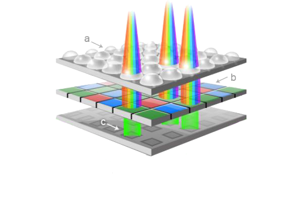
Bayer matrix of a color image.
What you have to keep in mind is that an RGB image and a B&W image are no longer directly compatible in the formulas due to their structure.
PixelMath #
- The operation of PixelMath is independent of any other process in progress, but also of any image or sequence previously loaded.
- However, when the desired operation is applied, the result is directly displayed in the preview window, ready to be saved. The default filename is ’new empty image'.
- PixelMath only supports the FITS format. It’s a choice. It is therefore useless to try to load TIFFs directly, for example. On the other hand, Siril knows how to read this latter format very well, so the solution is to open the TIFF file, save it in FITS, PixelMath-ise it, then save the result in the desired format.
- In the formulas applied by Pixel Math, keep in mind that the images are variables between 0 and 1. They are not normalized to 2n-1.
- The maximum number of images that can be used simultaneously is set to 10. You will see that this is already enough.
- The images used by PixelMath can be linear or not. However, to play live with the different layers, the linear version will be more visually adequate.
Graphic interface #
Here is an overview of the user interface:
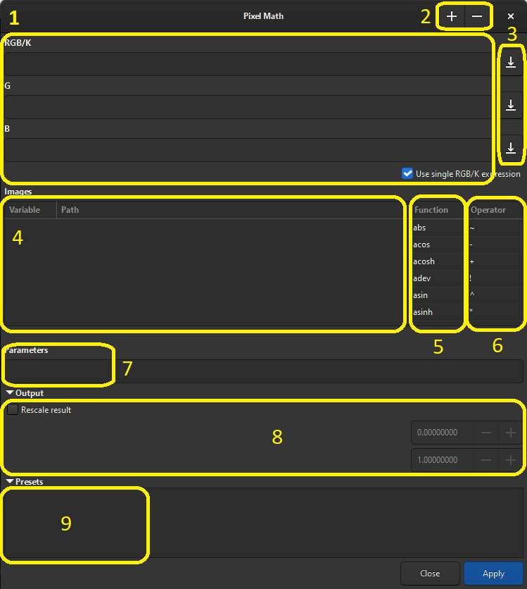
overview of the user interface.
- zone 1: This is the composition of our image, in 1 or 3 channels. If the image is in RGB format, only the top field (RGB/K) is accessible. To do this, the “Use a single RGB/K expression” box must be checked (otherwise an error message is displayed).
- zone 2: Allows you to add one (or more) image(s) or remove them from the list. The
+opens a standard window where multiple selection of files is possible. The-removes the highlighted variable from the list. It is essential that the images to be added are of the same type (number of channels) and of the same dimensions (WxH in pixels). Otherwise, an error message is displayed. - zone 3: 3 arrows to let you save individualy the formulas in an internal library (see zone 9).
- zone 4: List of usable images, divided into
Variables(variable name modifiable by double click) andPath(file location). - zone 5: All of the usable functions are described below.
- zone 6: All the operators also described below.
- zone 7: Field reserved for parameters (if used). See below.
- zone 8: To rescale the pixel of you image by a coefficient (one for low one for high).
- zone 9: The list of your preset functions.
Functions and Operators #
The various functions are almost all taken from the standard library. Operators can be either algebraic or logical.
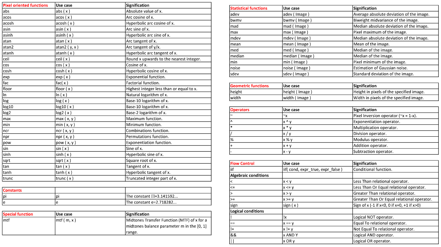
The different functions and operators.
A cheat sheet in PDF version is available here .
The special function “iif” #
This test function, aimed at flow control, has the following structure:
iif(condition, expression_if_True, expression_if_False)
- condition is a logical expression relating to a parameter or a variable.
- expression_if_True is then the result returned if the test is positive.
- expression_if_False is then the result returned if the test is negative.
For example:
Let’s take myPict1, a 3-channel image (RGB therefore).
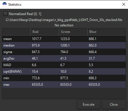
Statistics for RGB image myPic1.fits.
Here we have R=[772.6, 65535], G=[977.5, 65535] and B=[698.3, 65535] (because the image is in 16bit here, so max=65535).
Or, written otherwise, R=[0.018, 1], G=[0.015, 1] and B=[0.010, 1] (normalized to 1).
By applying the following condition:
iif(myPic1>0.2, myPc1, 0.1)
This leads to clipping to 6553.5 (=65535 x 0.1) the pixels of the image myPic1 whose values are less than 13107 (=65535 x 0.2).
For pixels whose value is greater than 13107, their value remains unchanged: this can be seen very clearly on the new values of the statistics.
Note that this reasoning is true for the 3 channels simultaneously.
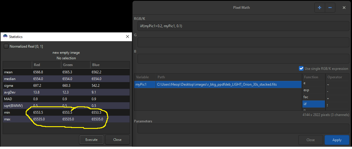
Statistics for RGB image myPic1.fits after PixelMath
The very special function “mtf” #
This function allows you to stetch the image. It requires 2 arguments:
- first, a parameter, in the range [0, 1].
This is the midtones value you would change with the appropriate slider in the Histogram Transform window.
This parameter can be either a constant decimal value or a predifined parameter as defined in zone 7.
- then the variable name of the image to be stretched. The target image can be RGB or BW.
So finally, the syntax would be:
mtf(myImageVariable, stretchValue)
Rescale #
By checking Rescale result, all the pixels of your image will be modified (rescaled).
For instance,
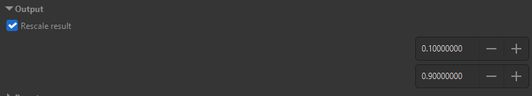
Rescale parameters example
In this case, the lower clipping value for each pixel of the image will be 6553.5 (0.1 x 65535), and the higher clipping value will be 58981.5 (0.9 x 65535).
Name of the variables #
By default, the variables are named I1 to I10, but you can customize these names, by double clicking on them. However, certain rules must be observed:
- character strings allowed
- alphanumeric strings allowed
- cannot contain only numbers
- no special characters, even at the beginning, except for
_ - no space
- case sensitive
Here is an overview of the possible combinations:
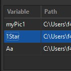
Different variable syntaxes allowed
Much more important: auto naming #
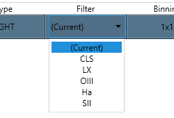
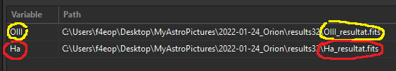
Under certain conditions, the name of each variable can be automatically assigned in a consistent way, to facilitate the identification and use of each variable. This is possible thanks to the use of the The FILTER= field in the header of the FITS file.
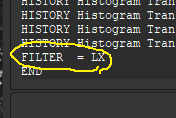
FILTER field in the Fits HEADER
There are several ways for this field to be automatically filled:
- with a correct configuration of your acquisition software (NINA, APT, …).
In this case, the header values will be kept as the conversion/preprocessDOF/alignment/stack operations progress.
We can thus find values like CLS, LX for color images, or OIII, Ha, SII for B&W. It is strongly discouraged to use any special character, even if your software allows it. However, special character
_is alowed.
The FILTER field in the Fits HEADER after NINA
- During an RGB, HaOIII, Ha or OIII extraction performed by Siril from a color image (OSC). Siril then fills the
FILTERfield of the header with the appropriate value.
The FILTER field in the Fits HEADER after an extractHaOII
Here is an example in pictures:
- A first image, whose FILTER field is empty, undergoes an RGB extraction under Siril.
- We then obtain 3 B&W files called
r.fits,g.fitsandb.fits. - A second image, whose FILTER field is
FILTER=LX(for example for L-Extreme), also undergoes an RGB extraction under Siril. - We then obtain 3 B&W files called
rr.fits,gg.fitsandbb.fits.
We then import the 6 B&W files to compare the auto-naming.
Next…in video:
The parameters #
Just like in math, these are integer or decimal values, defined in zone 7. These parameters can be used interchangeably in any formula (RGB or B&W), thus adding flexibility to the use of formulas.
You can list there all the parameters to be used in the various equations.
This list can be, for instance, something like:
k=0.7, P=3
The syntax:
- The different parameters are separated by a comma
- The decimal separator is a point
- Alphanumerical strings, lowercase or uppercase, including any special caracters except
,and=. - Case sensitive
Pixelmath becomes scriptable #
As for Siril 1.2.0, the Pixelmath feature became scriptable and also CLI usable.
The general syntax is:
pm "expression" [-rescale [min max]]
A basic example in a script could be as follow:
Assuming the two images image1.fits and image2.fits are located in the current working directory, the following function:
pm "$image1$ * 0.5 + $image2$ * 0.5" -rescale 0.0 0.9
will average each pixel of the 2 images, and rescale these pixels in the range [0.0 0.9].
Note that rescaling is an option.
Some use cases #
You now have all the tools to use PixelMath. Let’s proceed with some examples:
Basic use #
- Example 1: RGB image manipulation
This simple example shows how to import an RGB image into PixelMath, apply a factor to it, and check the result.
- Example 2: RGB image manipulation
Example similar to the previous one, but with a set of R, G and B images. We also add the application of a parameter.
The applied formula,
k*R+~k*B
allows to generate a synthetic G layer after the use of a Dualband filter, for example.
- Example 3: Starless
Suppose we have an RGB image, as well as the starless version. It is then easy to generate the “Stars” file.
Advanced use #
- Example 4: Generate a pseudo mask (B&W)
In this example, we start from an RGB image. After extracting the R, G and B channels, we are going to make the mask from the R channel by playing on its histogram (the black must be very black, and the white must remain degraded).
- Part of the mask is removed to make it selective.
- The mask, which is in B&W, is applied via PixelMath to the 3 layers R, G and B, in order to “raise” the red of part of the image.
- The resulting “local” image is then added to the original image.
It’s up to you now!!!