Removing gradients
In this tutorial, suitable for all levels, we will discuss the processing of gradients present in astronomical images. Indeed, even when the images are taken under a Chilean sky, and this is the case for the image that we will be using to illustrate the technique, they can be degraded by a light gradient whose origin may vary.
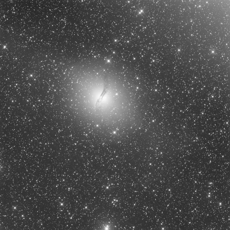
An example of light gradient, in the upper right corner, on an image taken under a Chilean sky.
Whether it is from light pollution from the nearby city, the Moon or any other light source, these gradients are unwanted signal that we would like to remove to create a better looking image. However, it is important to distinguish between a light gradient, whose origin is an external light source, and vignetting due to the optics. The latter, although it can be reduced with a gradient removal tool, is only perfectly corrected with the application of a master-flat.
Finally, this tutorial is intended for users with at least version 1.0.2 of Siril in which the tool has been completely revised, corrected and improved.
Removing a gradient from a stacked image #
The problem of removing the gradient often arises after stacking, when the addition of the pixels brings out the signal from the noise. Moreover, the gradient is not homogeneous from one image to another and the result accumulates all the individual gradients, making it more visible and complex.
Presentation of the tool #
The Background Extraction tool has two interpolation methods that are used in much the same way. The polynomial method and the RBF method, for Radial Basis Function. It is the latter that we will discuss in this section because it allows us to process more complex gradients using fewer samples. The tool window looks like this (open it from the Image Processing menu, Background Extraction… entry):
Presentation of the Siril background extraction tool.
- Two interpolation methods can be chosen.
- The first one, which has existed in Siril for many years, is the polynomial interpolation. It builds a synthetic polynomial sky background and works very well for simple gradients. The complexity of the corrected gradients is determined by the degree of the order of the polynomial used, the maximum being 4. The higher the degree the more complex the gradient. One of the advantages of this method will be described in the next section.
- The second method, RBF interpolation, is the one we will present in this tutorial, and the one we recommend to use in most cases.
- Smoothing is a parameter of the RBF interpolation that lowers gradients of the synthetic background. A smoothing parameter that is too small may result in overshoots and undershoots between background points, while a smoothing parameter that is too large may not be suitable for large gradient differences. It is recommended to try several values iteratively. The default value is 0.5.
- It is possible to generate a grid of points, called samples, automatically. This option defines how many samples to place on a horizontal line. The larger the number, the longer it will take to compute the synthetic background.
- The tolerance of the grid is a parameter defining whether or not a sample is placed in the image. Indeed, it is necessary to avoid placing samples on stars and / or objects in the picture that do not belong to the sky background.
- Sometimes, when the dynamic of the image is insufficient to sample a visually continuous gradation of colors, it is possible that circles or colored lines appear. This is called posterization. The Add dither option will add random noise in the gradient to make level successions smoother and remove this unwanted effect.
- Pressing this button generates a sample grid automatically, taking into account the parameters discussed above. This is required before continuing.
- This button allows you to erase all the samples present on the image.
- It is possible to correct the gradient in two ways. Either by subtracting the synthetic sky background (generally recommended method) or by dividing it. The latter may be preferred in the case where we seek to compensate for a problem of flat image.
- This button applies the gradient correction. It is possible to run it as many times as you wish, to see different results from different parameters. Only the final version will be kept when you close the tool.
- These options allow you to apply the gradient correction to the entire image sequence as we will discuss in the next section.
The Show original image button #
Once you have generated the samples and computed the background, keep pressing the button will toogle the before/after views of your image for a fast evaluation wich is so usefull.

The button Show original image.
Use case #
The first reflex to have, and which allows you to properly see the gradient present in the image, is to switch to Histogram visualization mode. Thus, the image is visually very stretched and all the defects become visible. You can also use the false color mode for an even more dramatic effect.
An image with a particularly complex gradient as seen in autostretch mode. The same image viewed in histogram equalization mode. This time, the image in histogram mode is displayed in false color.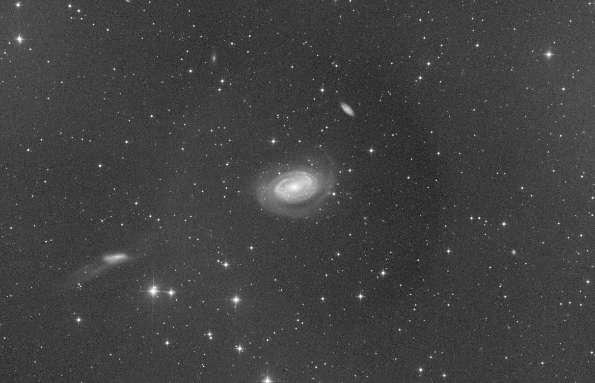
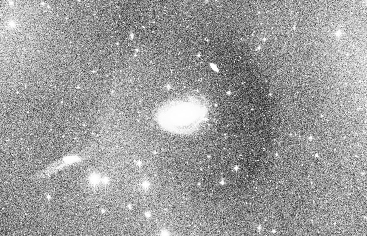
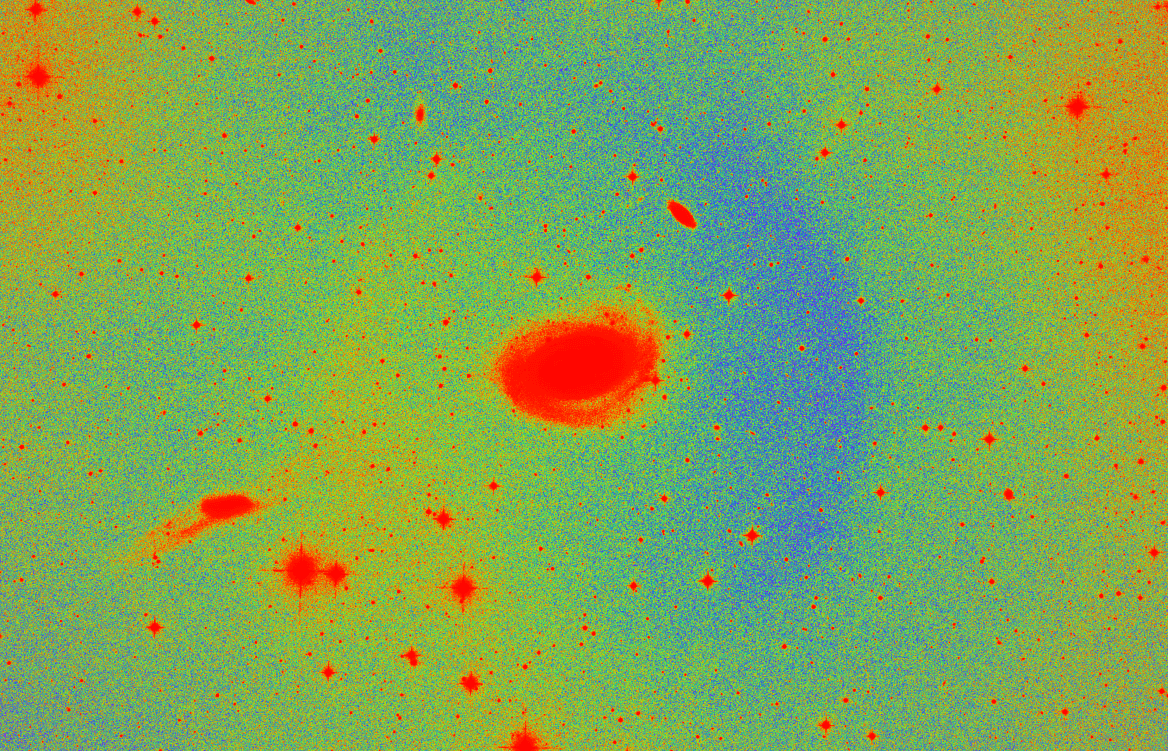
Then, it is possible to position the samples in two ways. Either manually or automatically as described above. To place them manually, left-click at the desired location on the picture and right click on a sample to delete it. The RBF interpolation does not require a large number of samples to be placed, which is why manual placement is the best option. It is also possible to combine the two methods, by laying a grid automatically and then adding/removing samples. However, a few rules must be observed:
- The samples are distributed over the entire image, taking care to place them only on the sky background.
- Avoid placing a sample on a large star compared to the sampling box.
Here, the position of the samples is chosen automatically to have a compact grid to try to correct the gradient. Pressing the 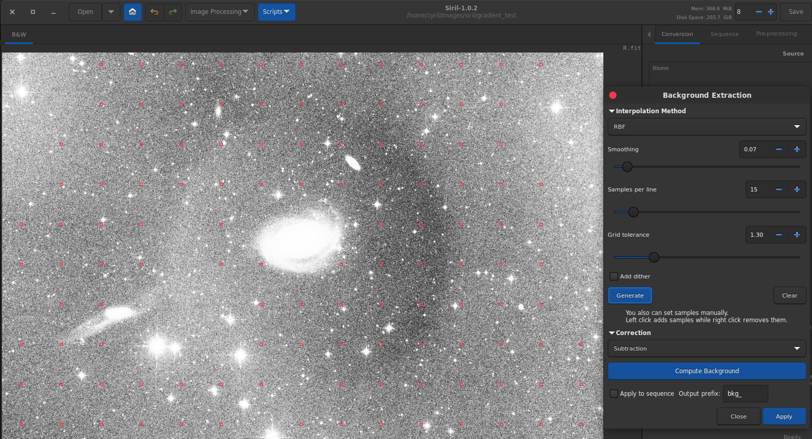
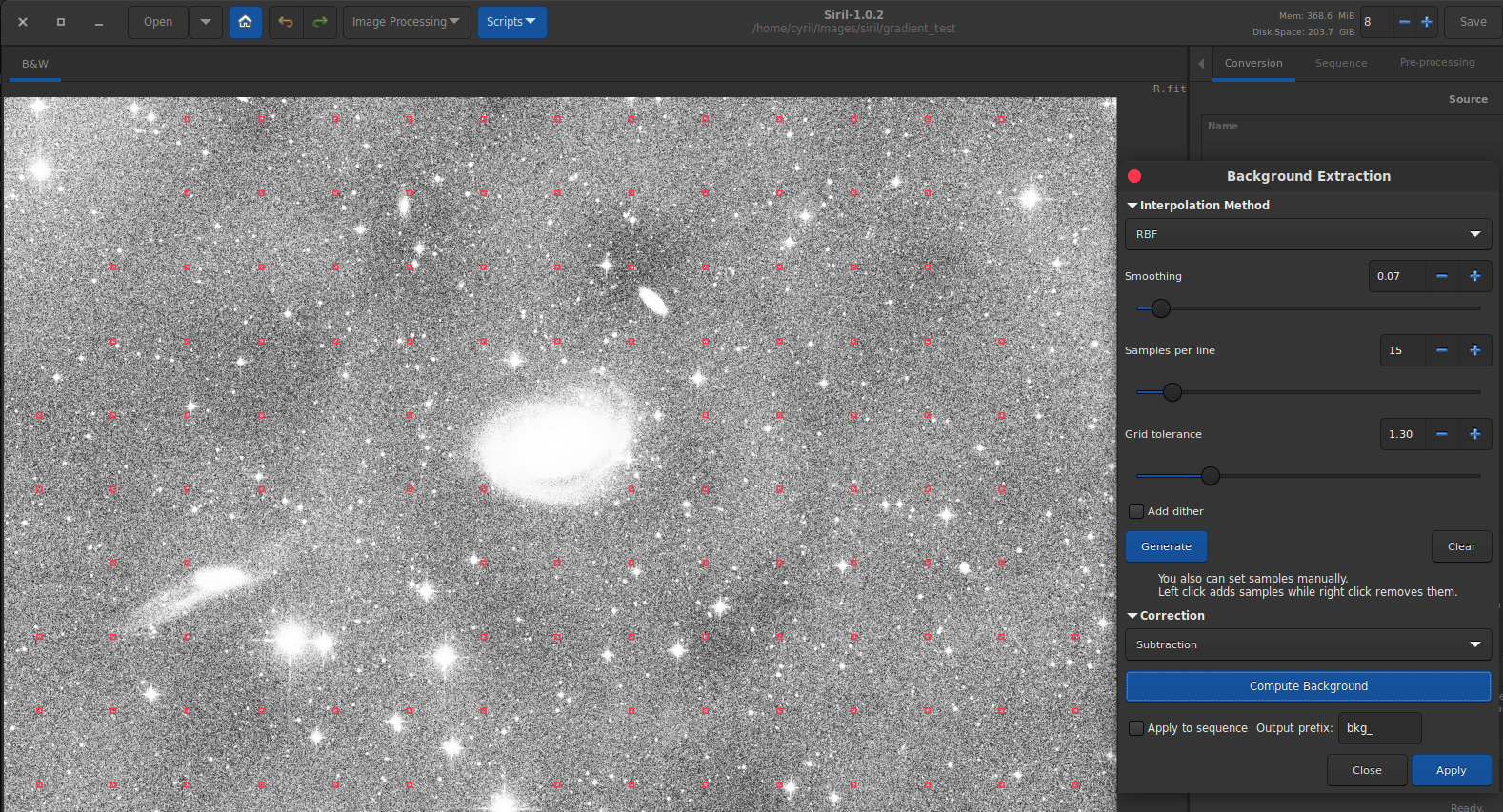
Compute Background button gives a first draft.
After choosing the samples, pressing the Compute Background button displays the result. This result is temporary and you have to click on Apply to validate it. However, as can be seen in the example image, even though most of the gradient has disappeared, some dark spots are still visible. Generally, this is due to the fact that some samples are placed on a star, or other object in the image. It is then sufficient to remove the sample that causes problems and restart the calculation. In this example, the smoothing was set to a quite low value in order to enhance this effect; however, be careful with the side effects of increasing it too much, which can lead to worse results.
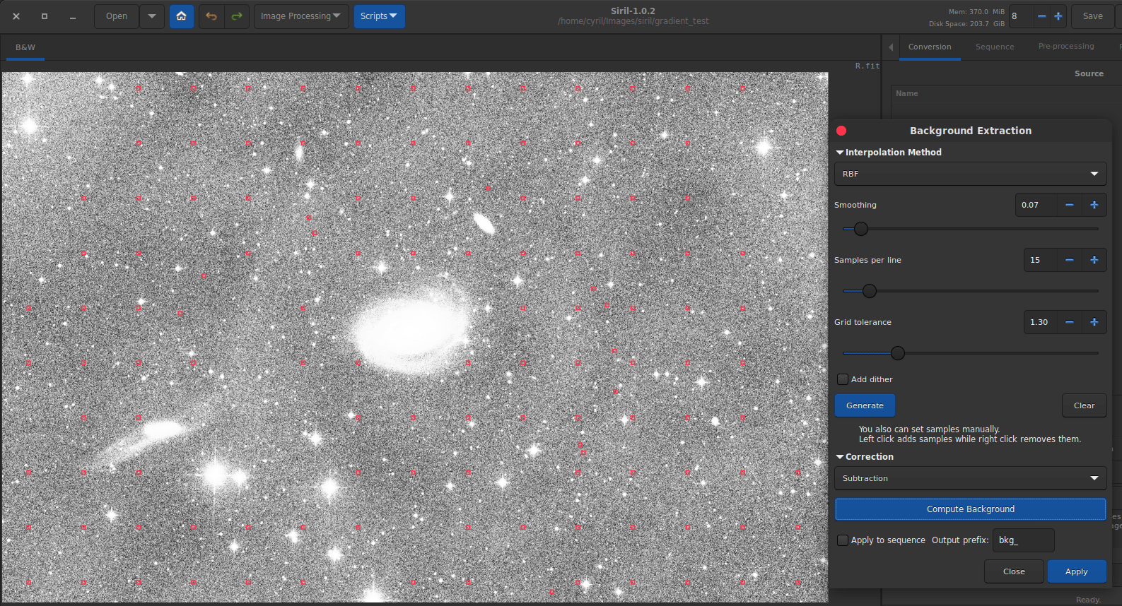
After several successive attempts, the result is as follows.
After some iterative work, the image above shows the result. Although not perfect, we can see that most of the gradient has been processed. Then we can press Apply to close the tool and return to our processed image. The Close button will cancel all changes of the tool and return to the original image.
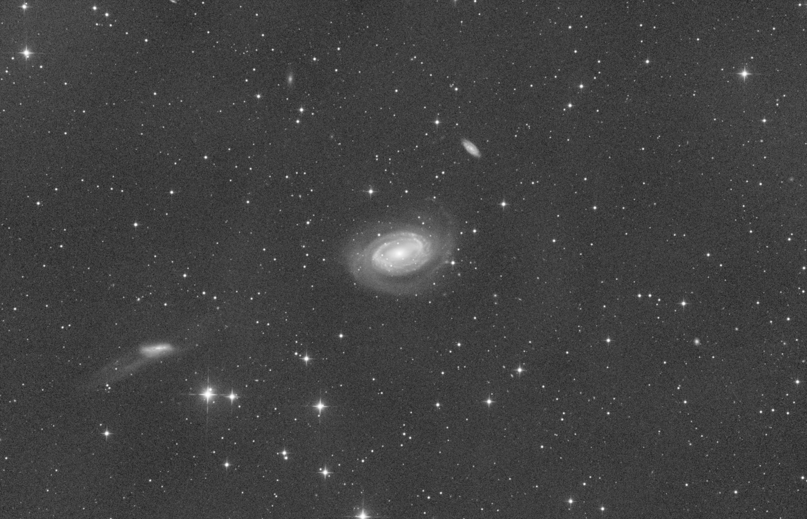
The same image seen in autostretch mode, the defects are now very little visible.
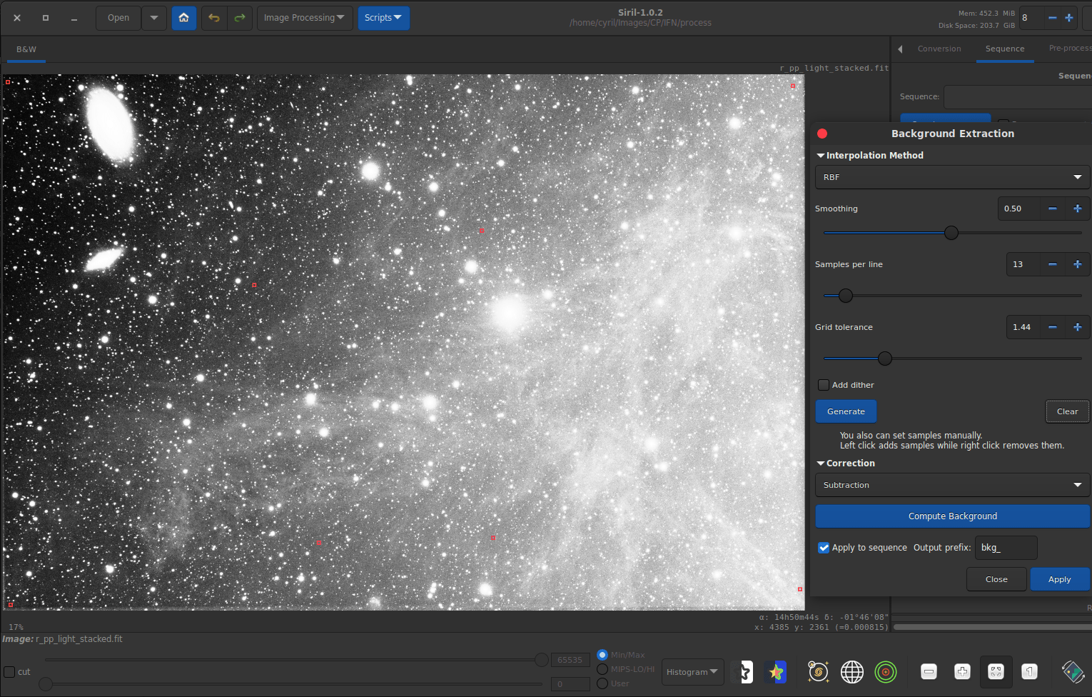
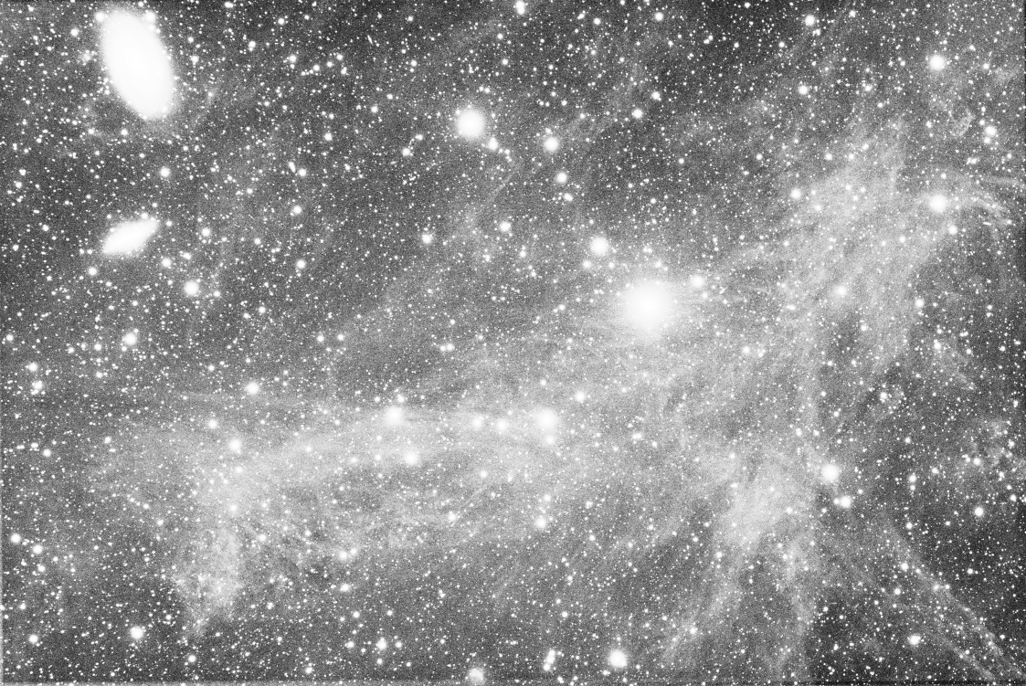
Here is an example where we try to remove light pollution. Only a few samples placed manually are then necessary.
Original image showing a strong gradient due to light pollution. Laying out the samples is very simple and only a few are needed (8 samples were used in this example). Click on the image to see more details. The result is completely free of the gradient and the IFNs become visible.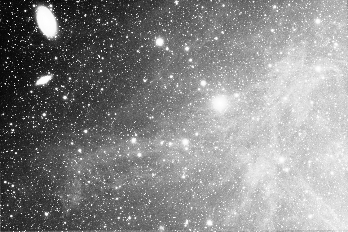
Removing a gradient from the images of a sequence #
It can sometimes be interesting to process the gradient on the individual images of the sequence. Indeed, the gradient of a stacked image is the sum of all the gradients contained in each image. Therefore, it may turn out that the gradient is very complex, sometimes too much, to be perfectly removed.
In this case, polynomial interpolation at the lowest degree (degree 1) is generally enough to correct these simple, often linear, gradients.
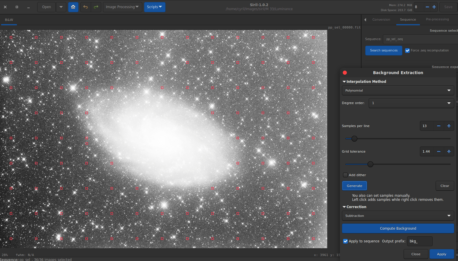
Here the background extraction is applied to each image of the sequence.
There is no need to click on Compute Background before applying: the grid and gradient are calculated for each frame. In the end, after stacking, the gradient to be corrected (if any) will be much easier to process.